The interface between protein and ligand
Binding affinity describes the strength of association between a ligand and its target protein. A binding structure records where the ligand sits within the protein. Our AGIMA-Score study asks which connections in that structure a model should learn from: every nearby atomic contact, or contacts across the binding interface?
Making the graph reflect the question
In panel D, edges connect protein atoms to ligand atoms. Distance ranges distinguish different neighbourhoods. The graph therefore emphasises how the two binding partners meet.
AGIMA-Score: learning intermolecular adjacency
Scoring protein-ligand binding structures through learning atomic graphs with inter-molecular adjacency ↗
Debby D. Wang and Yuting Huang
PLOS Computational Biology 21(5), e1013074 (2025)
From atomic contacts to a score
AGIMA-Score combines atom features with distance-dependent, intermolecular adjacency matrices. Graph convolutions and aggregation produce features used to estimate binding strength.
The study examines alternative atom-feature sets and adjacency definitions. The default model uses two intermolecular contact ranges: 2–3 Å and 3–4 Å.
The research code and trained model and data accompany the paper.
Testing on independent complex sets
Models were trained on PDBbind v2020 and tested on two CSAR sets. AGIMA-Score18 achieved the lowest test RMSEs in the comparison: 1.5806 and 1.6279. The eight-feature variant achieved the highest Test1 correlation, 0.7414.
Investigating what the model uses
Feature masking measures how validation performance changes when one feature type is removed. In the eight-feature variant, excluded volume has the largest effect.
UniMolRep addresses the complementary question of how representation combinations affect affinity prediction. See its PDBbind comparison for results using fingerprints, graphs and geometric features together.
Exploring grid-based scoring with GNINA
Our interactive exercise uses GNINA, a molecular docking package developed by McNutt and colleagues. It lets you examine how a three-dimensional grid of a protein–ligand complex becomes an affinity estimate.
Protein and ligand atoms occupy separate spatial channels. The crossdock_default2018 network produces an affinity estimate and a pose score. The two prepared examples are HIV-1 protease with MK1 (1HSG) and XK2 (1HVR).
a Prepared 1HSG complex
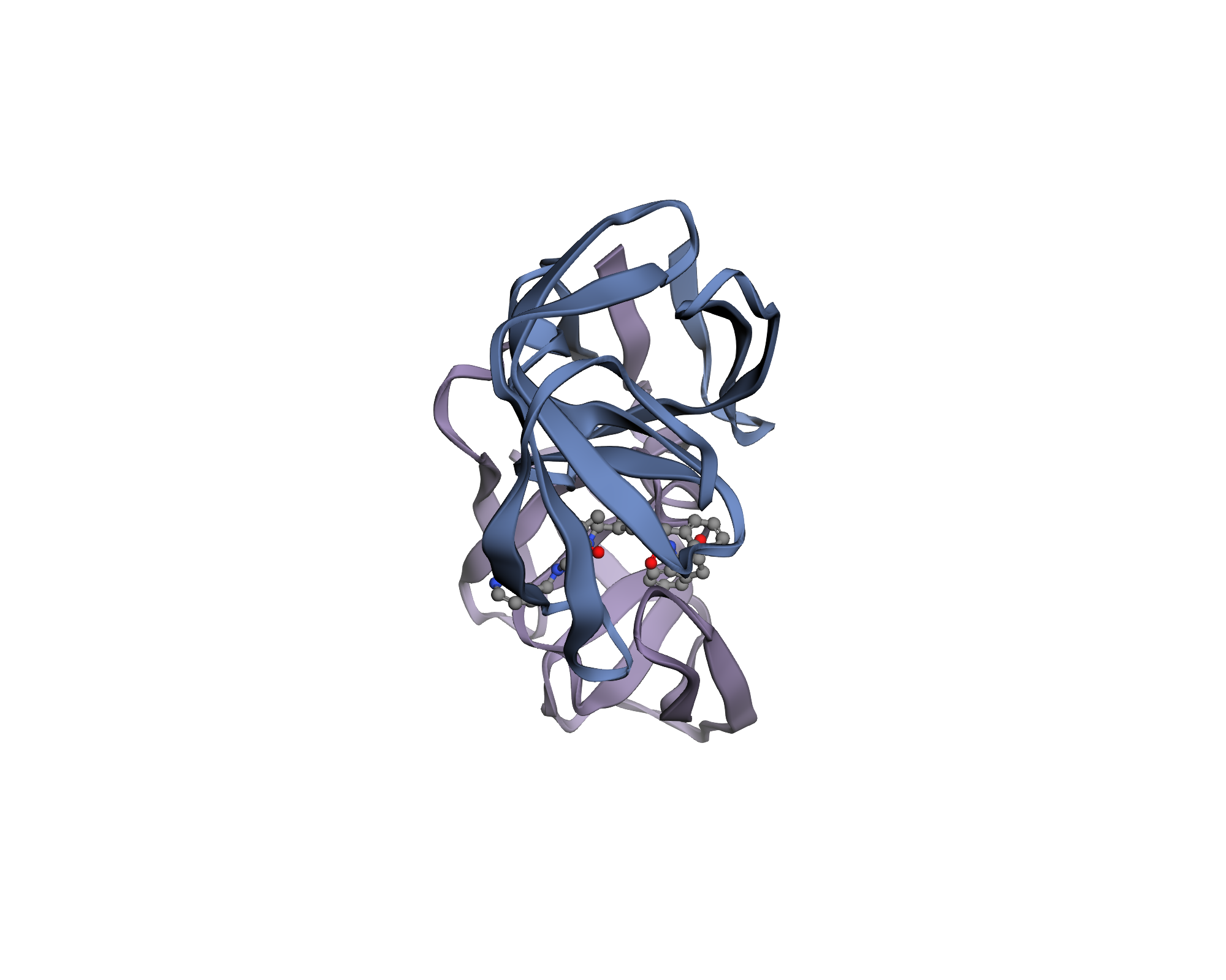
Protein and ligand retain their prepared coordinates.
b The MK1 binding pocket
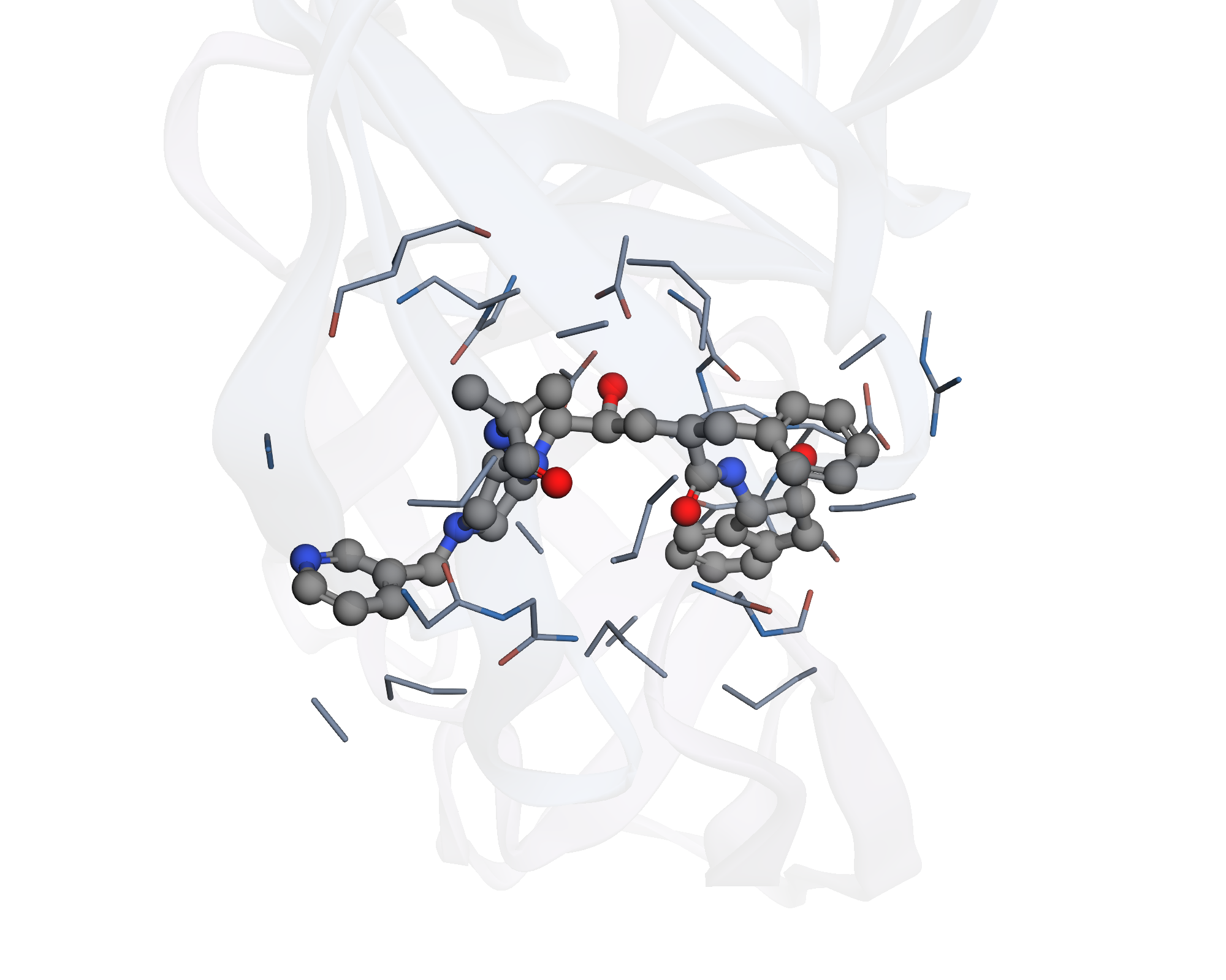
The enlarged view shows protein atoms within 5 Å of MK1.
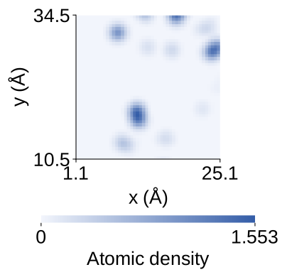
c Protein and ligand grids
Protein
Ligand
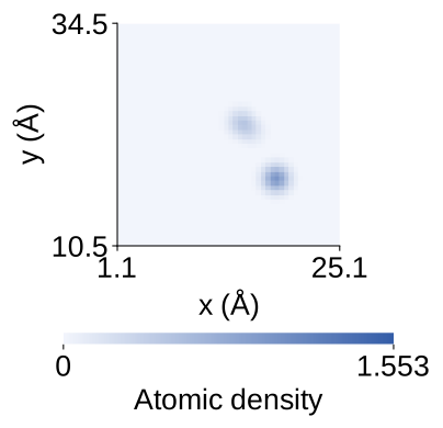
Two of 28 channels, on the same plane in a 24 Å field.
28 × 48 × 48 × 48 input 3D convolutions and pooling learned readouts
- Affinity estimate
- pK units; larger values indicate stronger predicted binding.
- Pose score
- CNNscore, from 0 to 1, assesses the supplied ligand arrangement.
The exercise scores the ligand in its supplied pose. Docking searches for candidate poses; rescoring applies an additional scoring model to those candidates.
What changes when a region is masked?
Spatial occlusion examines how a prediction responds when part of the input grid is hidden. All channels within one region are set to zero, while the molecular coordinates stay fixed.
Evaluate the masked grid with the same model, then subtract its score from the original score. Positive differences mean that masking lowered the estimate; negative differences mean that it raised the estimate. The comparison measures the model’s sensitivity to each region. [6]
a Keep the complex fixed
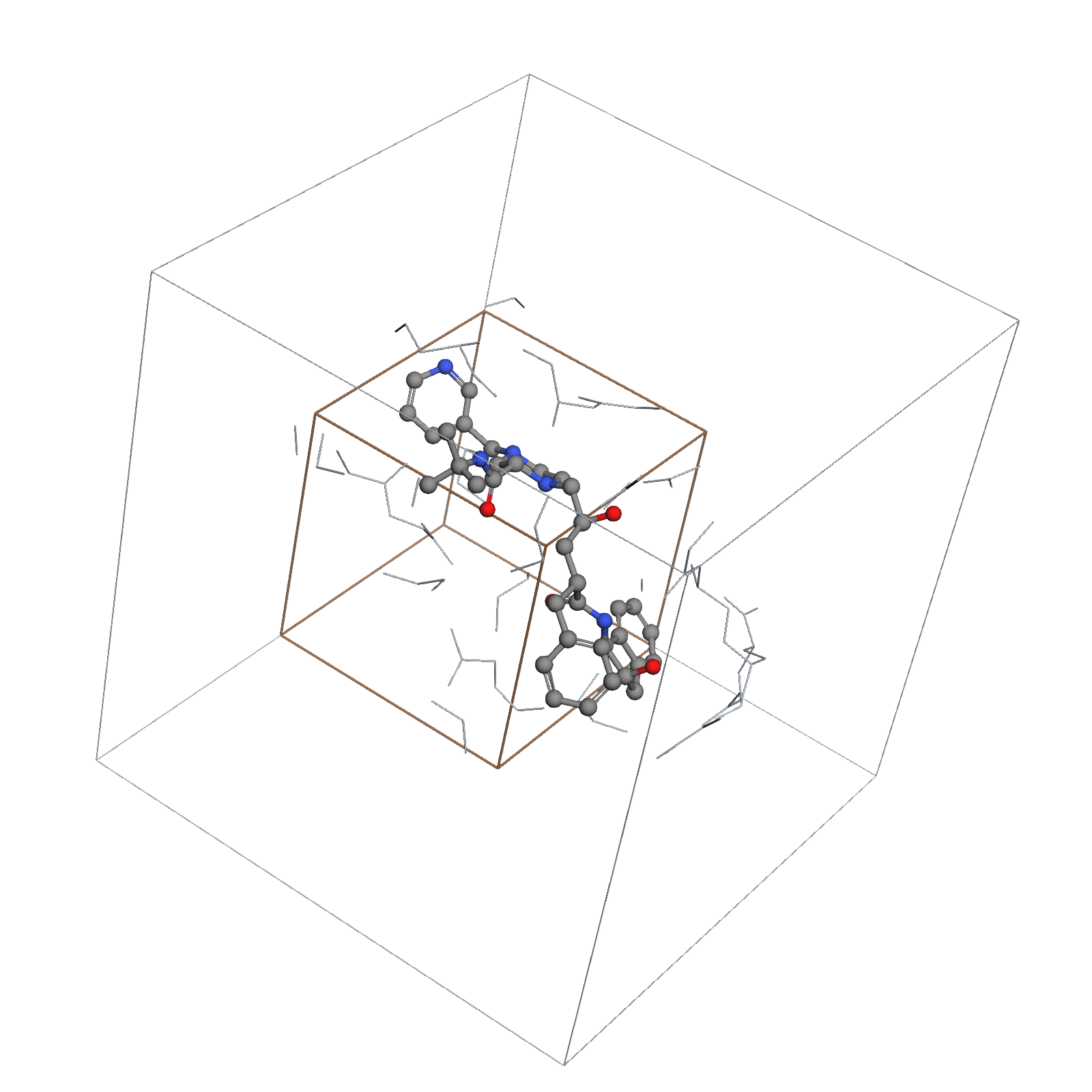
The ochre cube marks region A: the lower half of each grid axis. Ligand atoms retain their element colours; nearby protein atoms are shown as grey sticks.
b Original grid
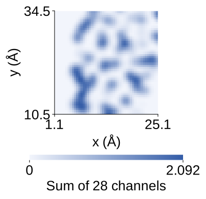
Evaluate the intact grid with GNINA.
c Masked grid
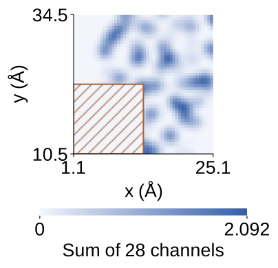
Zero all 28 channels in region A. Evaluate again with the same GNINA model.
Affinity scoring
Select a prepared complex and calculate its affinity and pose scores. Then choose Evaluate spatial occlusion to explore how masking different regions changes the affinity estimate.
Preparing analysis…
References
Debby D. Wang and Yuting Huang. Scoring protein-ligand binding structures through learning atomic graphs with inter-molecular adjacency. PLOS Computational Biology 21(5), e1013074 (2025).
Weiqing Guo, Jiawei Chen and Debby D. Wang. UniMolRep: A Python Package for AI-Oriented Molecular Representation Modeling. Journal of Chemical Information and Modeling (2026).
Andrew T. McNutt, Paul Francoeur, Rishal Aggarwal, Tomohide Masuda, Rocco Meli, Matthew Ragoza, Jocelyn Sunseri and David Ryan Koes. GNINA 1.0: molecular docking with deep learning. Journal of Cheminformatics 13, 43 (2021).
RCSB Protein Data Bank. RCSB Protein Data Bank: 1HSG. Protein structure record (1996).
RCSB Protein Data Bank. RCSB Protein Data Bank: 1HVR. Protein structure record (1995).
Matthew D. Zeiler and Rob Fergus. Visualizing and Understanding Convolutional Networks. Computer Vision – ECCV 2014, Lecture Notes in Computer Science 8689, pp. 818–833 (2014).