A model for one protein target
Screening asks which compounds to prioritise from a collection. In our study, a target-specific model learns from compounds labelled for one protein. It uses the ligand’s sequence and geometry to rank compounds by predicted activity against that target.
Why use two descriptions?
A SMILES sequence records chemical connectivity, while a molecular grid provides spatial context. Our question was whether learning interactions between these descriptions improves the ranking of active compounds.
DL-FSG: learning across two molecular views
Deep learning on the fusion of chemical sequences and molecular grids for ligand-based virtual screening ↗
Rongji Ke and Debby D. Wang
BIO Web of Conferences 232, 02002 (2026)
DL-FSG encodes the SMILES sequence and ligand grid in parallel. Bidirectional cross-attention lets the features from each branch inform the other. The combined features then produce a target-specific screening score.
Screening across 102 DUD-E targets
DL-FSG distinguishes active compounds from decoys with an AUROC of 0.9910 and an AUPRC of 0.9725 on the DUD-E benchmark.
What changes when a component is removed?
Replacing cross-attention with self-attention reduced AUC to 0.9855. Using either SMILES or grids alone also reduced performance. The two ablation studies support learning from both representations and their interaction.
Reading the grid branch with Grad-CAM
Grad-CAM highlights spatial regions associated with a higher screening score. It uses score gradients to weight the grid branch’s feature maps. The gradients pass through the sequence–grid fusion model while the molecule and conformer remain fixed. [2]
Follow the score back to the grid
The DL-FSG architecture joins sequence and grid features. Differentiate that joint score with respect to the grid branch’s spatial activations, before pooling and projection.
L = ReLU(Σk αkAk)
Ak is a spatial feature map. Its weight αk is the mean score gradient over that map. Only the positive part of the weighted sum is retained.
For this ethanol conformer, the MAO-B score is 0.5371.
a Locate the plane
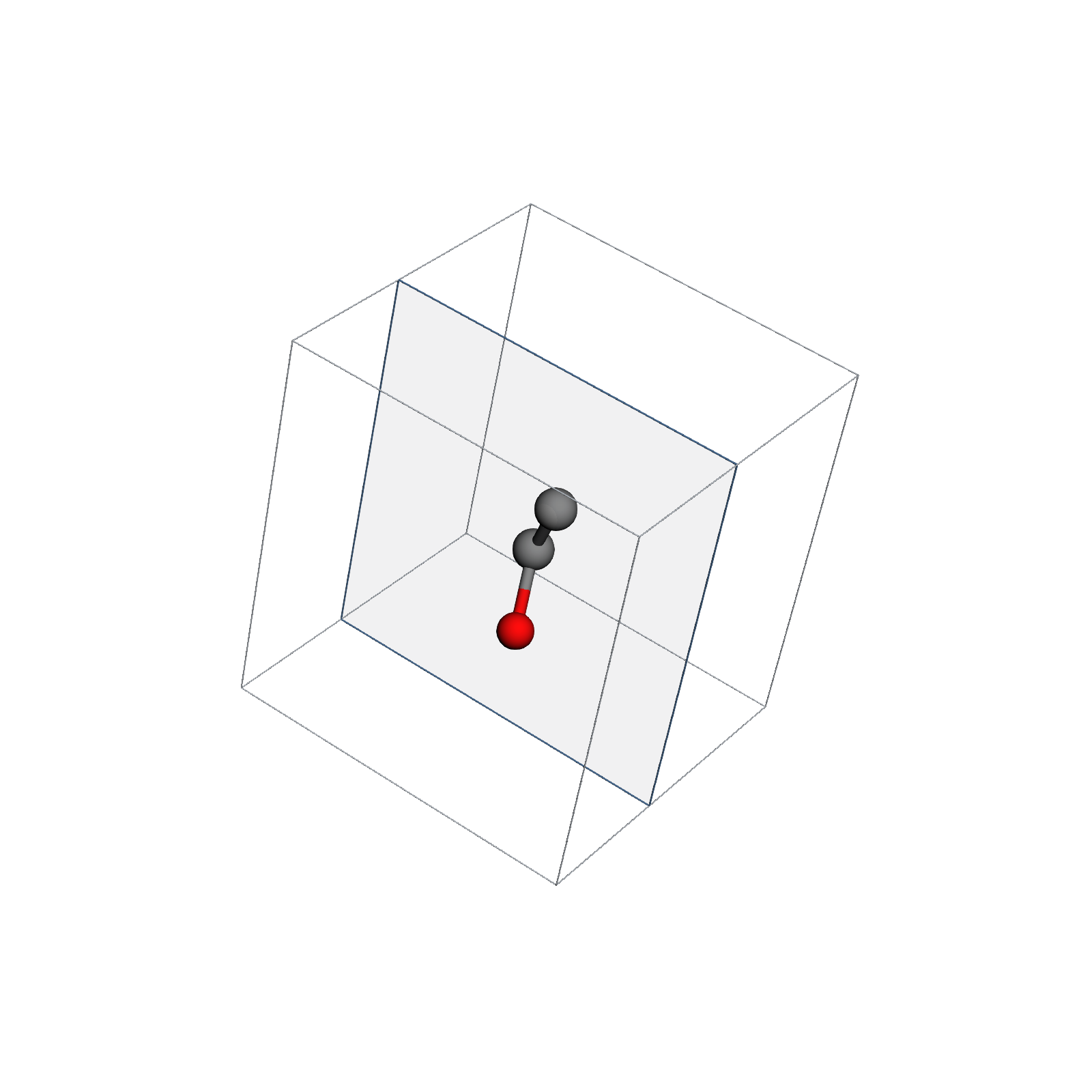
z = 0.21 Å in the model’s spatial frame.
b Read the spatial response
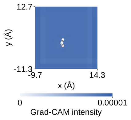
Atoms are projected onto the plane. The 24 Å field contains a 12 × 12 cross-section.
Each voxel summarises a spatial neighbourhood, giving a coarse view of the model’s response. Read the map at this scale rather than as a contribution from an individual atom. A shared colour scale allows comparisons across molecules.
Screening analysis
Try the MAO-B screening model with an example molecule or your own SMILES sequence. Its score ranks molecules for this target; it is not a calibrated probability of activity. After calculating a score, choose Calculate Grad-CAM to explore the spatial response.
Preparing analysis…
References
Rongji Ke and Debby D. Wang. Deep learning on the fusion of chemical sequences and molecular grids for ligand-based virtual screening. BIO Web of Conferences 232, 02002 (2026).
Ramprasaath R. Selvaraju, Michael Cogswell, Abhishek Das, Ramakrishna Vedantam, Devi Parikh and Dhruv Batra. Grad-CAM: Visual Explanations From Deep Networks via Gradient-Based Localization. Proceedings of the IEEE International Conference on Computer Vision, pp. 618–626 (2017).